 January
30
January
30
Tags
The Magic of a Memory Model
You know that moment when you can’t quite remember a song, but the instant it starts playing, the memory floods back and you can sing along perfectly? This last year the Nobel Prize in Physics was awarded to John Hopfield who came up with an elegant model for how this process could work in the brain, called a Hopfield Network (Hopfield, 1982). To see why this is worthy of a Nobel Prize, let’s first refresh our memories (no pun intended) of how memory works in a computer. In a traditional digital computer, there is a central processing unit (CPU) that follows explicit instructions (a program) to access memory. Memory is stored as bytes (8 bits – 1’s and 0’s) and each byte of memory has an associated address – the place on the drive where the memory is stored. This idea is a bit like needing to know the exact shelf a book is on in the library. Storing memories like this works great for computers but this kind of memory is not biologically plausible. In our brains, there is no evidence for a central planner that grabs bytes of memory, and yet we know our brains can store and retrieve memories. How we achieve this is a key question in neuroscience.
Learning
The trick which won John Hopfield the Nobel Prize, was to imagine that instead of having a fixed physical location for a memory, like a computer, memories could be stored in the way neurons are connected. To see how this works, let’s start with a simple example. Imagine we have four neurons, we can mathematically represent each one as either connected (1) or disconnected (-1) from other neurons in the network. Let’s see how we can store a simple memory pattern: on, off, on, on [1, -1, 1, 1]. You could also think of this as remembering directions as a right turn, a left turn, and then two right turns. To store this memory in the connections of neurons, we can borrow a famous idea from neuroscience; ‘neurons that fire together, wire together’. This concept is known as Hebb’s rule. In our example pattern, neurons 1,3, and 4 are on together, and so they should wire together positively (encourage each other to be on), whereas neuron 2 is off when the others are on, so we should discourage that neuron from being on when the others are on.
Looking at Figure 1, we can see Hebb’s rule in action. Neurons (rows) that are supposed to be “on” together form positive connections (as indicated by the entry in the corresponding column) and neurons that are off together form negative connections. For instance, neuron 1 has connections [0, -1, 1, 1], 0 because there are no self connections, -1 because if neuron 2 is on then neuron 1 should be off and vice versa, and the final two 1’s represent that if neuron 1 is active, then neurons 3 and 4 should be active. In other words, the neurons that fired together, wired together.

Figure 1: Gif of the learning rule for Hopfield Networks. Each element of the pattern (p) gets multiplied by every other element of the pattern. The result of that multiplication tells each neuron (the rows of the matrix W) whether or not it should be active with each other neuron.
Energy and Memory Recovery
Storing a pattern is only half the battle – we also need to recover it. Think back to our song example: when you hear part of a familiar tune, these stored connections between notes help you recall the rest. The way this works, according to Hopfield, is a bit like an avalanche. When one note gets played a neuron which responds to that note will get triggered and then that triggers the neurons, which, in the past were active with that first neuron and so on until it no longer makes sense to trigger any more neurons. This process looks a lot like a ball rolling down a hill, so we may use the metaphor of energy. When the neural pattern is far away from a stored memory, energy is high (like the ball being at the top of the hill) as the pattern gets closer and closer to a memory it reaches the bottom of a ravine – its figurative energy is lower, and there is nowhere else for it to move and we have arrived at our memory, we remembered!
It’s not only simple patterns the network can store. Take this image of the number four which we will have a Hopfield Network remember (Figure 2).
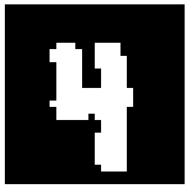
1 (white) or -1 (black). It was originally hand drawn, and grey scale (each pixel
can only be 0-255, from black to white) but in order to get it to work with a
Hopfield Network, we have to threshold the image, if a pixel is below 255/2 set
the pixel to -1 and if it’s above set it to 1. There are alternative Hopfield
Networks which can work with continuous data (Ramsauer et al., 2021), but
these binary ones were the first and are the nicest for expository purposes.
Of course, images are two-dimensional, each pixel has 2 coordinates, and our model only takes in one-dimensional patterns. To get around this we can just flatten the image. If the image was originally a 25×25 table it is now a 625 (25×25 = 625) element list of 1’s and -1’s. Now that we have stored it, it’s time to see what the network can do. We can present this corrupted image (figure 3), like a fragment of a song, to our model and see if it can recover the initial memory. Figure 4 is an animation showing the network doing just that, remembering the full image. On the left is an animation of the memory process; at each time step we select one of the pixels and ask if flipping it would increase or decrease the energy of the system (Figure 4; right), If it decreases the energy then we flip the pixel, if it increases the energy then we keep it the same. If flipping any of the pixels will only increase the energy then we know we are done and we have found the stored memory.
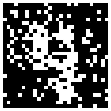
20% of the elements were randomly selected
and their entries were flipped by multiplying their values by -1.
The idea is that at each step I am either flipping or not flipping an entry based on if it will minimize the energy of the system like a ball rolling down a hill. We have stored our pattern- our memory- as an energy minimum of our system through the connectivity of our neurons. This is much more biologically plausible than the digital computing model of memory- instead of needing an exact address we can use even a partially complete copy of the original memory (like a part of the song).
Conclusion
Hopfield Networks also have their faults. In a network with N neurons, you can only store 0.14N patterns. This is quite low – for example, with 100 neurons, you can only store 14 patterns. Each neuron added only lets you store 0.14 more patterns. Since the 80’s there has been big improvements on the storage capacity of these networks, some (Krotov & Hopfield, 2016) have exponential storage capacity, but at the end of the day, Hopfield Networks are cool not because of what they can do, but how they do it.
Appendix
Learning rule
We can be slightly more precise. If we define a memory, p, as a string of bits of length N, then we can encode this memory using a special matrix (our network), we’ll call it W (of size NxN), which encodes connections between model neurons. Each neuron has a row (indexed by the letter i) and a column (indexed by the letter j). The connection between neurons is given by their respective indices. For instance, if I wanted to know what the connection was between neuron i and neuron j I would look at entry ij. The matrix is symmetric (i.e. W(i,j) = W(j,i)), off diagonal (i.e. W(i,i) = 0) , and each element can only be -1 or 1. To memorize our memory we use a simple rule, Wij = pi pj. Let’s do an example: Given pattern p = [-1,1,1,1], we need a matrix W of size 44. Because the matrix is symmetric we don’t need to start with what goes in W11, let’s start with W12. First we look at what’s in the pattern at position 1 and multiply it by what is at position 2, W12 = -1 1 = -1. Instead of working through the rest of what the matrix should be, I’m going to have Python do it; W = np.outer_product(p,p), that’s it!. The learning rule of the Hopfield Network exactly (minus the zeros on the diagonals) corresponds to an outer product of a pattern with itself. After doing that we get:
W = [ 0, -1, -1, -1],
[-1, 0, 1, 1],
[-1, 1, 0, 1],
[-1, 1, 1, 0]
Update Rule
In this matrix, our memory is encoded! We just need some way of getting that memory out. The way this will work is we will input some memory, then we will use some rule which will tell us what to do with that memory. The key idea here is that the relationships between the neurons have already encoded our memory, we just need some way of extracting it. The learning rule is set up in such a way that if two neurons are not active together they will get opposite signs (𝑖.𝑒. −1×1=1×−1=−1) and if they are active together they will get the same sign (𝑖.𝑒. −1×−1=1×1=1). Thus we want an update rule which will tell us what neuron i should be given its weights with all the other neurons and the current value of the other neurons. What about this, we sum the multiplication of each learned weight from neuron i to j with the pattern at j. This will tell us to be either the same as or the opposite of whatever j is, summed over all j’s. We can write that like this:
pi = 1 if Σj Wijpj> 0
Else, pi = -1.
Energy
Take a little leap with me and imagine that why this works is that the update step is minimizing energy. Energy in this sense means something like, distance from equilibrium. Each neuron wants to push or pull all the other neurons and the sum of all those forces is equal to our energy. Actually as a matter of fact the energy of a hopfield network can be written as a summation:
E = -1/2 Σi Σj Wijpipj
For a second ignore the -1/2 and the outer summation, let’s focus only on the Σj Wijpipj. Note for a second that this looks suspiciously like our update rule Σj Wijpj except this time we are including the pattern’s value at index i. What this is doing is summing over the connections to neuron i, then multiplying each one by the current value of the pattern at i and j. Let’s step even further into the equation and only look at what’s going on with pipj The idea here is that we are asking whether or not neurons i and j agree. Agreement is either -1 -1 or 1 1disagreement is the opposite and will always be -1. Now remember what Wij represents, it encodes the relationship between neurons i and j. Let’s take the case where Wij=1 (i.e. these neurons are supposed to agree). If they agree then the term in the summation is positive and that will contribute negatively (because of the leading minus sign) to the energy function. The inverse is also true, if they disagree when they are supposed to agree then that will contribute positively to the energy function. The opposite of all that happens when Wij= -1.

You must be logged in to post a comment.